
Satellite Data for Precision Agriculture: Variable Rate Application and Yield Optimization
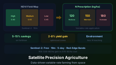
Quick Answer: Precision agriculture uses within-field variability maps — primarily from satellite NDVI — to apply inputs (fertilizer, water, pesticides) at variable rates matched to crop needs. The workflow: satellite NDVI map → management zone delineation → soil sampling by zone → prescription map → variable rate application via GPS-guided equipment. Sentinel-2 at 10m resolution provides sufficient detail for most field-scale applications. Economic benefit: variable rate lowers input use by cutting over-application, and can raise yield where the input being varied was the limiting factor — so the payoff scales with how variable the field is and how much over-application there was to begin with, and a strip trial against the uniform rate is the only reliable way to size it on a given farm. Key limitation: satellite NDVI shows current crop status but doesn't directly indicate the cause of variability (nutrient deficiency, water stress, soil compaction, pest damage all reduce NDVI similarly). Ground-truthing remains essential.
Precision agriculture uses satellite vegetation maps to apply fertilizer, water, and pesticides at variable rates matched to what each part of a field actually needs — turning within-field variability from a hidden cost into a managed one. A 200-hectare wheat field isn't uniform. The north end has heavier clay soil that holds more water. The southeast corner has a sandy rise that drains quickly and stresses crops in dry spells. The center strip along the old creek bed has deep, fertile topsoil. Applying the same fertilizer rate everywhere — 150 kg/ha of nitrogen uniformly — means over-fertilizing the productive zones and under-fertilizing the stressed areas.
Satellite imagery makes this within-field variability visible, enabling farmers to match inputs to actual crop needs at each location. This is the core of satellite-enabled precision agriculture.
Why does crop growth vary within a field?
Crop growth varies within a field because soil, topography, water availability, and management history all change over short distances — one corner drains fast and stresses in dry spells, another holds water and stays productive. Traditional farming ignores this and applies uniform rates everywhere, which over-treats the strong zones and under-treats the weak ones. The main drivers:
Soil variation: Texture, organic matter, depth, drainage, pH, and nutrient content vary across fields — often dramatically over short distances.
Topography: Hilltops lose soil and water; depressions accumulate both. Slope aspect affects solar exposure and evapotranspiration.
Water availability: Irrigation non-uniformity, drainage patterns, and water table depth create variable moisture conditions.
Management history: Previous crop rotations, tillage practices, and input application patterns create legacy effects.
This variability means that a uniform management approach is suboptimal everywhere — too much input in some areas, too little in others.
The Satellite-to-Prescription Workflow
Step 1: Satellite Vegetation Map
Acquire a Sentinel-2 image during active crop growth (typically mid-season when biomass differences are most apparent):
- Calculate NDVI (or a more specific index like NDRE — Normalized Difference Red-Edge — which is more sensitive to nitrogen status)
- The resulting map shows within-field crop vigor variation at 10m resolution
Step 2: Management Zone Delineation
Convert the continuous NDVI map into discrete management zones:
- High-vigor zone: NDVI > 0.75 — crop is performing well; current management adequate
- Medium-vigor zone: NDVI 0.55-0.75 — moderate performance; potential for improvement
- Low-vigor zone: NDVI < 0.55 — crop is stressed; investigation needed
Typically 3-5 zones per field, delineated using clustering algorithms (k-means) applied to multi-year NDVI maps (to separate persistent patterns from single-year anomalies).
Step 3: Targeted Soil Sampling
Instead of random soil sampling across the field, sample strategically within each management zone:
- 3-5 soil samples per zone
- Test for nitrogen, phosphorus, potassium, pH, organic matter
- Results represent the soil condition specific to each zone's performance level
Step 4: Prescription Map
Combine satellite zone map with soil test results to generate a variable rate prescription:
| Zone | NDVI | Soil N Status | Prescribed N Rate |
|---|---|---|---|
| High vigor | 0.80 | Adequate | 120 kg/ha (reduce) |
| Medium | 0.65 | Low-moderate | 150 kg/ha (maintain) |
| Low vigor | 0.45 | Very low | 180 kg/ha (increase) |
The prescription map is loaded into the GPS-guided variable rate applicator.
Step 5: Variable Rate Application
GPS-guided equipment (fertilizer spreader, sprayer, seeder) reads the prescription map and adjusts application rate in real-time as it traverses the field:
- Total input may be the same as uniform application
- But distribution is optimized — more where needed, less where not
- Result: more uniform crop performance, better resource efficiency
Multi-Temporal Monitoring
A single satellite image captures one moment. Season-long monitoring provides richer information:
Growth curve analysis: Track NDVI development from planting through harvest. Areas that fall behind early may need different intervention than areas that decline late in the season.
In-season adjustment: Mid-season satellite imagery can prompt supplemental fertilizer applications to zones that are underperforming.
Year-over-year comparison: Consistent low-vigor zones across multiple years indicate persistent soil or drainage problems requiring structural solutions (tile drainage, liming, organic matter building) rather than just increased fertilizer.
Which Vegetation Index?
No single index is right for every stage — matching the index to the job is part of the workflow. The common choices:
NDVI: The most widely used. Good general indicator of crop vigor and biomass. Limitation: saturates at high biomass (LAI > 3-4), making it less useful for distinguishing among healthy, high-biomass crop areas.
NDRE (Normalized Difference Red-Edge): Uses Sentinel-2's red-edge band (B5, 705nm) instead of visible red. More sensitive to chlorophyll/nitrogen variations in dense canopy. Better for mid-to-late season nitrogen management in high-biomass crops.
MSAVI (Modified Soil-Adjusted Vegetation Index): Reduces soil background influence. Better for early-season monitoring when canopy cover is partial and soil is visible between rows.
LAI (Leaf Area Index): Derived from multiple bands. Directly relates to canopy structure. Available as a Sentinel-2 biophysical product.
Why is Sentinel-2 the go-to satellite for precision agriculture?
Sentinel-2 is the go-to satellite for precision agriculture because it combines 10-meter resolution, a 5-day revisit, chlorophyll-sensitive red-edge bands, and free open access — a mix no other public mission matches. One pixel covers 100 m², enough to map within-field variation on fields larger than about 5 hectares. The specifics:
10m resolution: One pixel covers 100 m² — sufficient to map within-field variability for fields larger than ~5 hectares.
5-day revisit: Frequent enough to track crop development and respond to emerging stress.
Red-edge bands: B5 (705nm), B6 (740nm), B7 (783nm) provide chlorophyll and nitrogen-sensitive information unavailable from Landsat.
Free access: No data cost, enabling routine monitoring throughout the growing season.
Does precision agriculture pay off?
Often, but the honest answer is that it depends on the field, and anyone quoting you a single percentage is selling something. The economics are not mysterious — they are just specific to your situation. Where the value comes from:
Input cost reduction: Variable rate lowers total input use by cutting application in zones that were being over-treated under a uniform rate. The saving therefore scales with how much over-application there was to begin with. A field that is genuinely uniform, or one already managed at a lean rate, has little to recover.
Yield improvement: Redirecting input toward under-performing zones can lift yield, but only where the limiting factor was the input you are varying. If the low-vigour zone is limited by compaction or drainage instead of nitrogen, more nitrogen buys nothing — which is why the diagnosis gap below matters so much.
Environmental benefit: Reduced over-application decreases nitrogen leaching, runoff, and greenhouse gas emissions. This benefit is real even in the cases where the on-farm financial return is marginal.
Return on investment: The satellite imagery itself is free (Sentinel-2). The real costs are GPS-guided variable rate equipment, the agronomic advice needed to turn a vigour map into a defensible prescription, and the time to run it. On operations that already own compatible equipment, the marginal cost is small and the case is straightforward; where the equipment has to be bought for this purpose, the payback period is the thing to model, not the per-hectare saving.
The only reliable way to know what it is worth on a specific farm is a strip trial: run variable rate against the uniform rate on the same field in the same season, and measure the difference with the yield monitor. Published trial results vary widely by crop, region, and baseline practice, so they indicate direction rather than a number you can bank.
Limitations
Diagnosis gap: Satellite NDVI shows WHERE the crop is stressed but not WHY. Low NDVI could mean nitrogen deficiency, water stress, soil compaction, pest damage, disease, or herbicide injury. Ground investigation is needed to determine the cause before prescribing a remedy.
Temporal gaps: Cloud cover prevents satellite observation on many dates during the growing season, potentially missing critical growth stages. In cloud-prone regions, this is a significant practical limitation.
Resolution vs. field size: 10 m pixels work well once a field is big enough to contain plenty of pure interior pixels — from roughly 5 hectares upward, as above. Below that, mixed edge pixels make up too much of the field for reliable zoning, and the smaller fields common in many developing countries need higher resolution: either commercial satellite imagery or drone-based mapping.
Adoption barriers: Variable rate technology requires GPS-guided equipment and technical knowledge. Adoption rates vary enormously: high in large-scale operations (US, Australia, Brazil), low in smallholder agriculture.
Precision agriculture is one of the few satellite applications where the benefit lands on an individual end-user rather than being diffuse or public: most remote sensing value accrues to society, but a variable-rate prescription shows up on one farm's own input bill and yield monitor. That directness is what makes it measurable — and what makes it worth measuring on your own fields rather than taking on faith. The same season-long vegetation maps also feed yield estimation, closing the loop from in-field monitoring to harvest forecast.

Remote sensing specialist with 10+ years in satellite data processing and AI. Founder of Off-Nadir Lab. Ph.D. in Informatics (Yokohama National University, 2026). Master's in Earth System Science and Technology (Kyushu University). Co-author, Remote Sensing Encyclopedia. More about the author →