
InSAR: How Satellites Measure Millimeter Ground Movement from 700 km Up
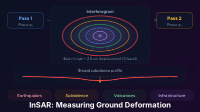
Quick Answer: InSAR compares the phase of radar signals from two SAR acquisitions over the same area. If the ground moved between acquisitions, the path length changes, producing measurable phase shifts. One full phase cycle (2π) corresponds to half the radar wavelength of ground displacement — about 2.8 cm for Sentinel-1's C-band. With advanced processing (PS-InSAR, SBAS), millimeter-per-year deformation rates are detectable. Applications include earthquake co-seismic displacement, volcanic inflation, land subsidence from groundwater extraction, and infrastructure stability monitoring.
InSAR detects ground movement by comparing the phase of radar signals between two SAR acquisitions of the same area. A displacement of just half the radar wavelength — 2.8 cm for Sentinel-1's C-band — produces a full cycle of phase change, and time-series methods push detection limits down to millimeters per year.
That sensitivity is why Mexico City has become the standard illustration of what InSAR can do — not because of an earthquake, but because of groundwater extraction slowly compacting the clay lake bed the city is built on. InSAR observations spanning 2014–2021 put the sinking at roughly 35 centimetres per year, unevenly distributed across the basin. The subsidence is invisible at ground level (too slow, too uniform), but from space the deformation pattern is unmistakable. No other measurement technique captures ground movement that subtle at that scale.
How Does InSAR Work?
InSAR works because SAR records not just the intensity of the returned radar signal — the brightness values that most SAR analysis is built on — but also its phase: the position of the wave within its cycle when it returns to the satellite. Comparing the phase of two acquisitions over the same area reveals tiny changes in the satellite-to-ground distance, and therefore any ground movement between the two passes. As NASA Earthdata's SAR primer puts it, "InSAR uses the phase information recorded by the instrument to measure the distance from the instrument to the target."
Phase is sensitive to that distance with extraordinary precision. A change in distance of just half the radar wavelength produces a full cycle of phase change. For Sentinel-1's C-band (5.6 cm wavelength), half a wavelength is 2.8 cm. If the ground moves 2.8 cm between two satellite passes, the phase shifts by exactly 2π (one full cycle).
Interferometry compares the phase from two SAR acquisitions. Subtracting the phase of one image from the other produces an interferogram — a map of phase differences that encodes:
- Topographic phase: Height differences cause phase differences (this is how SAR-derived digital elevation models are created)
- Deformation phase: Ground movement between acquisitions
- Atmospheric phase: Variations in atmospheric delay between the two dates
- Noise: Random phase contributions from temporal surface changes
The goal of InSAR processing is to isolate the deformation signal from the other components.
Differential InSAR (DInSAR)
The simplest InSAR approach subtracts the topographic phase contribution (using a known DEM) to isolate the deformation signal:
Deformation phase = Total phase − Topographic phase − Atmospheric phase − Noise
The result is a map of colored fringes, where each fringe (complete color cycle) represents one half-wavelength of ground displacement in the satellite's line-of-sight direction.
How Do You Read an Interferogram?
Fringes are the language of interferograms: each complete color cycle represents one half-wavelength of line-of-sight displacement (2.8 cm for Sentinel-1). Fringe spacing tells you the deformation gradient, fringe shape points to the deformation source, and counting fringes gives total displacement. The characteristic patterns:
- Widely spaced fringes: Gradual deformation over a large area (regional subsidence)
- Tightly packed fringes: Rapid deformation gradient (fault rupture, localized collapse)
- Concentric fringes: Radially symmetric deformation (volcanic inflation/deflation, sinkhole)
- No fringes: No detectable deformation (or complete decorrelation)
The direction of the color cycle (e.g., blue→green→red) indicates whether the ground moved toward or away from the satellite. Convention varies by software, so always check the sign convention. If you're still getting comfortable with radar imagery in general, our practical guide to reading SAR images covers the amplitude side of the story.
What Is Coherence, and Why Does It Matter?
Coherence measures whether the ground surface stayed stable enough between acquisitions to maintain a consistent phase relationship — the precondition for InSAR to work at all. It ranges from 0 (completely random phase — no useful signal) to 1 (perfect phase preservation). Every interferogram comes with a coherence map, and reading it tells you where the deformation measurements can be trusted.
High coherence areas:
- Urban buildings, infrastructure, bare rock
- Arid terrain with minimal surface change
- Stable agricultural land (between growing seasons)
Low coherence areas:
- Dense vegetation (leaves and branches move between passes)
- Water surfaces (constantly changing)
- Snow-covered areas (melting and accumulation)
- Construction zones (surface physically altered)
In tropical forests, C-band coherence can drop below usable levels within days. This is why L-band systems (like ALOS-2 PALSAR and NISAR) are preferred for InSAR in vegetated areas — the longer wavelength penetrates deeper into the canopy and maintains coherence longer.
Coherence loss is a nuisance for deformation mapping, but it's a signal in its own right: coherence change detection exploits sudden coherence drops to map building collapse, flooding, and other surface disturbance.
Time Series InSAR: PS-InSAR and SBAS
Single interferograms are limited by atmospheric noise, which can mimic or mask real deformation. Time series approaches solve this by combining many interferograms:
Persistent Scatterer InSAR (PS-InSAR)
Identifies pixels that maintain high coherence across all acquisitions in a stack (typically 20-50+ scenes spanning 1-2 years). These "persistent scatterers" — usually buildings, rocks, or infrastructure — provide reliable phase measurements that can be analyzed as a time series.
The atmospheric contribution varies randomly from scene to scene but is spatially smooth within each scene. The deformation signal is temporally smooth but can vary spatially. By exploiting these different statistical properties, PS-InSAR separates the two.
Result: A deformation time series at each PS point. Because atmospheric noise averages down as scenes accumulate, the velocity of a long-lived scatterer can be resolved far more finely than any single interferogram allows — millimetres per year is the commonly quoted regime. The precision actually achieved on a given site depends on stack length, scatterer quality, and how well the atmosphere was modelled, so it should be reported per project rather than assumed.
Small Baseline Subset (SBAS)
Instead of requiring persistent high coherence, SBAS combines interferograms with short temporal and spatial baselines to maximize the number of usable pixels. This produces lower precision per pixel but much better spatial coverage, especially in semi-vegetated areas.
Real-World Applications
Earthquake Deformation
The 2023 Turkey-Syria earthquakes produced meters of horizontal displacement along the fault rupture. InSAR mapped the co-seismic deformation field within days of the event, revealing the fault geometry and slip distribution. This information fed directly into seismic hazard models — and the same SAR acquisitions supported rapid building damage assessment through coherence change.
Land Subsidence
Groundwater extraction, mining, and oil/gas production cause the ground to compact and subside. InSAR monitors this across entire cities and regions (we cover the workflow in detail in our ground subsidence monitoring guide):
- Jakarta: Severe subsidence concentrated in the northern coastal districts
- Mexico City: On the order of tens of centimetres per year, with the fastest rates in the former lake bed
- San Joaquin Valley, California: Extensive agricultural pumping subsidence
Volcanic Monitoring
Magma moving toward the surface inflates the volcanic edifice, producing a characteristic pattern in InSAR. Regular monitoring can detect pre-eruptive inflation months before surface activity begins. Multiple volcano observatories worldwide now include InSAR as a standard monitoring tool.
Infrastructure Monitoring
Buildings, bridges, dams, and railway lines all experience slow deformation that can indicate structural problems. PS-InSAR time series detect:
- Differential settlement of buildings
- Thermal expansion cycles
- Slope instability affecting transport infrastructure
- Dam deformation
InSAR by Application: Matching Method to Problem
Matching the InSAR method to the application means matching the deformation's magnitude and spatial scale to what a single interferogram, or a stack of them, can resolve. There is no universal detection threshold — what you can measure at a given site is set by the coherence you get there, the length of the stack, and how well atmospheric delay can be separated from real motion. The table below is a routing guide, not a specification:
| Application | Deformation magnitude | Recommended Method | Key Constraint |
|---|---|---|---|
| Earthquake co-seismic displacement | Centimetres to metres, in one step | DInSAR | Phase unwrapping fails where fringes are too dense to count |
| Volcanic pre-eruptive inflation | Millimetres to centimetres per month | DInSAR, time series | Atmospheric noise, severe in tropical settings |
| Urban subsidence (e.g., Jakarta, Mexico City) | Centimetres per year, sustained | PS-InSAR | Needs a long stack of acquisitions per site |
| Tectonic interseismic creep | Millimetres per year | PS-InSAR, SBAS | Long time series (multiple years) needed |
| Infrastructure differential settlement | Sub-millimetre to millimetres per year | PS-InSAR | Requires high persistent-scatterer density |
| Mining-induced subsidence | Centimetres to metres per year | DInSAR, SBAS | Phase unwrapping over a steep subsidence bowl |
| Landslide slow creep | Millimetres per month | SBAS | Temporal decorrelation on vegetated slopes |
| Permafrost seasonal frost heave | Centimetres per season | DInSAR | Seasonal baseline only (summer) |
Wavelength and coherence: The wavelength sets both the sensitivity and how long coherence survives, and the two trade against each other. C-band (Sentinel-1, 5.6 cm) suits urban and arid areas where the surface stays stable between passes. L-band (NISAR, ~24 cm) penetrates vegetation canopy and holds coherence longer in forested terrain, which is why it is preferred where C-band decorrelates. X-band (~3 cm) gives the finest displacement per fringe — half a wavelength, so roughly 1.5 cm — but decorrelates fastest of the three. For a large continental earthquake such as the 2023 Kahramanmaraş sequence in Türkiye, Sentinel-1 interferograms mapped metre-scale co-seismic displacement across the whole rupture within days, which is the property that makes InSAR valuable for rapid response: coverage of the entire deformation field, not a denser network of points.
What Are InSAR's Limitations?
InSAR's main limitations are geometric and environmental: it measures only line-of-sight displacement, loses coherence over vegetation and water, and can confuse atmospheric delay with real deformation. Processing is also demanding — phase unwrapping, orbit precision, and DEM quality all shape the result. None of these is fatal, but each determines where and how InSAR can be applied reliably.
Line-of-sight measurement: InSAR measures displacement along the satellite's look direction, not purely vertical or horizontal. Decomposing into 3D deformation requires combining ascending and descending orbits.
Temporal decorrelation: In vegetated areas, coherence drops rapidly. C-band InSAR over forests is often limited to winter (leaf-off) periods.
Atmospheric artifacts: Turbulent atmosphere, especially in mountainous areas, creates phase patterns that resemble deformation. Time series analysis mitigates but doesn't fully eliminate this.
Ambiguity: Phase wraps every 2.8 cm (for C-band). Deformation larger than this per fringe cycle requires "unwrapping" — an algorithmic step that can fail in areas of rapid deformation or low coherence.
Processing complexity: InSAR processing is significantly more demanding than standard SAR analysis. Free tools like ESA's SNAP toolbox handle the standard interferometric workflow, but orbit precision, DEM quality, co-registration accuracy, and atmospheric modeling all affect the result.
Despite these limitations, InSAR remains the only technique capable of measuring ground deformation across hundreds of kilometers with millimeter precision, at regular intervals, without any ground-based equipment. For geoscientists, civil engineers, and hazard analysts, it has fundamentally changed what questions can be asked — and answered — about how the Earth's surface moves. And if you want to explore the Sentinel-1 archive that underpins most InSAR work, our Sentinel-1 SAR viewer is a quick way to browse acquisitions over any area of interest.

Remote sensing specialist with 10+ years in satellite data processing and AI. Founder of Off-Nadir Lab. Ph.D. in Informatics (Yokohama National University, 2026). Master's in Earth System Science and Technology (Kyushu University). Co-author, Remote Sensing Encyclopedia. More about the author →