Forest Degradation vs. Deforestation: Why Detecting Degradation Is Harder
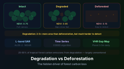
Quick Answer: Deforestation — complete conversion of forest to non-forest — is relatively easy to detect from satellites because NDVI drops dramatically and the spectral signature changes from vegetation to bare soil or crops. Degradation — partial removal of trees through selective logging, fire damage, or fragmentation — is much harder because the canopy may close within months and spectral changes are subtle. Yet degradation is now the larger disturbance by area: a satellite study covering the whole Brazilian Amazon found 337,427 km² degraded between 1992 and 2014 against 308,311 km² deforested, and its cumulative carbon emissions may rival those from outright clearing. Detection approaches include SAR texture analysis (canopy gaps from logging), time series anomaly detection (temporary NDVI dips), and high-resolution canopy gap mapping. L-band SAR is more sensitive to degradation than C-band because it detects biomass loss in the trunk layer.
Deforestation is easy to see from space and degradation is not — that gap is the whole story. Complete forest clearing produces an unmistakable spectral jump from vegetation to bare soil that any sensor can catch, while selective logging or understory fire removes only part of the canopy, which often closes over the gaps within months. And degradation is not a marginal problem: across the Brazilian Amazon it has affected more area than outright clearing, so the form of forest loss satellites struggle most with is also the more widespread one.
When most people think of forest loss, they picture the dramatic images: bulldozers pushing trees into piles, vast cleared areas visible from space. That's deforestation — complete removal of forest cover — and satellites have been detecting it effectively for decades.
But there's a quieter, more insidious form of forest loss that satellites struggle to see: degradation. A logging operation that removes 30% of the large trees from a tropical forest causes massive carbon loss, biodiversity damage, and ecological disruption — but from satellite altitude, the remaining canopy closes over the gaps within months, and the forest looks superficially intact.
This detection gap matters enormously. A satellite study of the entire Brazilian Amazon found that from 1992 to 2014, the total area of degraded forest was 337,427 km², compared with 308,311 km² that were deforested — degradation is now a larger disturbance by area than clearing, and its cumulative carbon emissions may rival those from outright clearing. Yet most global forest monitoring systems primarily detect deforestation, not degradation.
The Detection Challenge
Why is deforestation easy to detect?
Deforestation flips a pixel from one clear spectral state to another. Intact forest shows high NDVI, strong near-infrared reflectance, and complex canopy texture; cleared land shows low NDVI, bright visible reflectance from exposed soil, and a smooth surface. That contrast is large enough for even coarse sensors to catch, which is why the transition is so straightforward to map:
- Before: High NDVI (0.6-0.8), high NIR reflectance, complex canopy texture
- After: Low NDVI (0.1-0.3), high visible reflectance (bare soil), smooth texture
This contrast is detectable by virtually any satellite sensor at any resolution. Even MODIS at 250m can detect deforestation of a few hectares.
Why is degradation hard to detect?
Degradation removes trees without removing the forest, so the spectral change is small and short-lived. Selective logging opens 10–30m canopy gaps that surrounding crowns close within months, NDVI may fall only 0.05–0.15 (inside the range of normal seasonal variation), and the logging roads and skid trails that give the operation away are often just 3–10m wide — below the resolution of medium-resolution sensors. Selective logging, for example, creates subtle changes:
- Canopy gap formation: Individual tree removal creates gaps that may be 10-30m across — smaller than many satellite pixels
- Rapid gap closure: In tropical forests, canopy gaps close within 3-12 months as surrounding trees expand their crowns
- Remaining canopy masks the signal: NDVI may drop by only 0.05-0.15 — within the range of natural seasonal variation
- Logging roads and skid trails: Narrow linear features (3-10m wide) that are below the resolution of medium-resolution sensors
The Temporal Window
For selective logging, the window of satellite detectability is narrow:
- Pre-logging: Intact forest canopy
- During/immediately after logging: Gaps visible, logging roads fresh, disturbed soil exposed
- 3-12 months later: Canopy closing, roads revegetating, spectral signature returning toward pre-disturbance
- 2+ years later: Canopy appears intact at medium resolution; only structural differences persist
If a satellite doesn't image the area during this brief window — or if clouds obscure the observation — the degradation event may never be detected.
Detection Approaches
High-Resolution Canopy Gap Mapping
At sub-meter to 5m resolution, individual canopy gaps from selective logging are visible:
- Gap size and distribution: Logged forests have more and larger gaps than undisturbed forests
- Logging road networks: Characteristic branching pattern of main haul roads and smaller skid trails
- Log landing areas: Cleared areas where logs are collected for transport
Commercial daily constellations at 3–5 m — Planet's, for example — enable gap-based degradation mapping, but require both a data licence and sophisticated automated analysis to handle the volume.
SAR-Based Detection
SAR offers advantages for degradation detection:
L-band (ALOS-2): Sensitive to biomass changes in the trunk layer. Selective logging removes large trees (reducing L-band backscatter) while the remaining canopy may mask the change in optical imagery. L-band SAR "sees through" the remaining canopy to detect the biomass loss below.
Canopy texture changes: SAR image texture changes when the forest structure is altered by logging. Metrics like gray-level co-occurrence matrix (GLCM) contrast and homogeneity differ between intact and selectively logged forests.
Coherence patterns: Logged forests may show different temporal coherence patterns than intact forests due to structural changes.
Time Series Anomaly Detection
Dense optical time series (Sentinel-2, Landsat) can detect degradation as temporary departures from the expected NDVI trajectory:
- Build a model of expected NDVI behavior for each pixel (seasonal pattern, inter-annual trend)
- Flag pixels where observed NDVI falls below the expected value by more than a threshold
- Classify the anomaly: magnitude and duration distinguish degradation from clouds, seasonal variation, and deforestation
CODED (Continuous Degradation Detection) and similar algorithms implement this approach, detecting both gradual degradation and abrupt deforestation from the same time series.
Multi-Spectral Change Metrics
Some spectral changes associated with degradation are more persistent than canopy closure suggests:
SWIR reflectance: Increases with canopy gap fraction and remains elevated longer than NDVI changes, because exposed soil and woody debris in gaps have high SWIR reflectance.
Red-edge bands: Sentinel-2's red-edge bands are sensitive to canopy chlorophyll content, which may remain reduced in degraded forests even after gap closure.
Canopy water content: Derived from SWIR bands; selectively logged forests may have lower canopy water content due to changed microclimate and edge effects.
Types of Degradation
Selective Logging
The most widespread form in tropical forests:
- Removes 1-10 trees per hectare (but each tree may be 50+ cm diameter)
- Collateral damage: for every tree harvested, 10-20 additional trees may be damaged
- Logging infrastructure (roads, skid trails) fragments the forest
- Detection: Gap mapping, SAR biomass change, logging road detection
Fire-Induced Degradation
Understory fires in humid tropical forests:
- Fire kills smaller trees and damages larger ones without consuming the canopy
- From above, the canopy appears intact but the forest structure is fundamentally altered
- Detection: Thermal anomaly detection during fire; post-fire SWIR/NBR changes; time series NDVI decline
Edge Effects and Fragmentation
Forest edges created by adjacent deforestation experience:
- Increased tree mortality (wind exposure, desiccation)
- Vine proliferation
- Structural simplification
- Detection: Buffer analysis around deforestation edges; biomass change detection in edge zones
Fuelwood and Charcoal Production
In many developing regions, forest degradation from fuelwood collection and charcoal production:
- Gradual thinning of forests near settlements
- Often below the detection threshold of individual satellite observations
- Detection: Long-term biomass trend analysis; nighttime light proximity analysis
Why is degradation undercounted in carbon accounting?
Degradation emissions slip through the cracks because the systems that measure forest carbon were built to track area, not quality. IPCC and national greenhouse gas inventories often undercount degradation because monitoring focuses on where forest disappears rather than where it thins, the term itself resists a consistent threshold, and the satellite limitations described above mean many events are never recorded at all. Specifically:
- Monitoring systems focus on deforestation (area change) rather than degradation (quality change)
- Degradation is harder to define consistently (what threshold of canopy loss constitutes degradation?)
- Satellite detection limitations mean much degradation goes unrecorded
Degradation is widely thought to account for a substantial share of forest-sector carbon emissions in tropical countries — a share that current monitoring systems largely miss, which is precisely why the published estimates disagree with each other so widely. An emission source you cannot observe consistently is an emission source you cannot bound.
Detection Limits: Degradation vs. Deforestation
Setting realistic expectations for degradation monitoring means being clear about which constraint binds for each sensor:
| Method | What it can realistically detect | Binding constraint |
|---|---|---|
| MODIS NDVI (250m) | Large clearings only | Pixel size — selective logging is invisible |
| Landsat NDVI (30m) | Clearings down to roughly the sub-hectare scale | Cloud cover; degradation only in the strongest cases |
| Sentinel-2 NDVI (10m) | Smaller clearings, faster confirmation | Canopy closure hides gaps within months |
| Sentinel-2 SWIR + red-edge | Partial-canopy loss, with careful analysis | Signal is small relative to seasonal variation |
| Sentinel-1 SAR (C-band) | Clearings through cloud, year-round | Saturates in dense canopy; degradation signal is indirect |
| L-band SAR (ALOS-2, NISAR) | Biomass loss beneath a closed canopy | Revisit frequency; data access and cost |
| Commercial 3–5 m optical | Individual canopy gaps and skid trails | Licensing cost and processing volume |
| GEDI LiDAR (spaceborne) | Canopy height loss | Sparse sampling — footprints, not wall-to-wall maps |
The emissions accounting gap: the reason degradation emissions are so poorly constrained is structural, not incidental. Events small enough or subtle enough to fall below the detection limits above never enter the record at all, so the observed total is a lower bound by construction, and the size of the shortfall is itself unmeasured. Estimates of degradation emissions from the same region can differ by a factor of several depending on which sensor and threshold the study used — which is the signature of a measurement problem rather than a disagreement about the forest.
Selective logging detection timing is the most critical operational consideration: ground disturbance from a logging operation — skid trails, log landings, fresh soil — is visible in high-resolution imagery only for a limited window before regrowth and canopy closure obscure it. Missing that window means the event is effectively unrecorded. Capturing it reliably requires both metre-scale resolution and near-daily revisit, a combination currently available only from commercial constellations, which is a significant part of why operational degradation monitoring lags deforestation monitoring.
Closing the Gap
Progress is being made:
Higher resolution, more frequent data: Planet's daily 3-5m imagery and Sentinel-2's 5-day revisit at 10-20m make the detection window for degradation more accessible.
L-band SAR: ALOS-2 and NISAR — the NASA-ISRO mission launched on 30 July 2025 — provide biomass-sensitive SAR data that detects degradation below the canopy.
AI/deep learning: Machine learning models trained on known degradation events are improving automated detection rates.
Integration: Combining optical time series, SAR biomass monitoring, and high-resolution gap mapping creates a multi-evidence approach where each method compensates for others' weaknesses. Knowing the forest type being watched sharpens every one of these methods, since expected trajectories differ between a conifer plantation and a tropical broadleaf stand — and running the comparison as a repeated change-detection task is what turns single observations into a monitoring record.
The distinction between deforestation and degradation isn't just a technical classification issue — it determines whether the full scope of human impact on forests is visible or hidden. Making degradation visible from space is essential for honest carbon accounting, effective forest governance, and meaningful progress on climate and biodiversity commitments.

Remote sensing specialist with 10+ years in satellite data processing and AI. Founder of Off-Nadir Lab. Ph.D. in Informatics (Yokohama National University, 2026). Master's in Earth System Science and Technology (Kyushu University). Co-author, Remote Sensing Encyclopedia. More about the author →