
Flood Monitoring with Sentinel-1 SAR Time Series: Tracking Inundation from Space
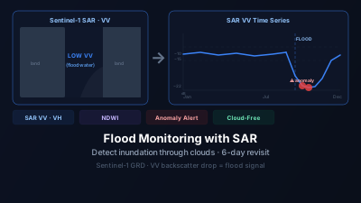
Quick Answer: Flooding causes a sharp drop in Sentinel-1 SAR VV backscatter: open water is smooth and reflects the radar signal away from the sensor, producing very low values. A sudden VV drop over a flat area — not explained by vegetation seasonality — almost always indicates inundation. By tracking SAR VV time series over a floodplain, river delta, or coastal zone, you can detect flood onset within one satellite overpass (6-day revisit), observe peak extent, and monitor recession over days or weeks — all through clouds, at night.
Why SAR Is the Right Tool for Flood Monitoring
Floods happen fast and are almost always accompanied by clouds. Optical satellites like Sentinel-2 cannot see through cloud cover — the very weather that causes flooding blocks the view. This is the core reason that Sentinel-1 SAR has become the primary satellite system for operational flood monitoring worldwide.
Synthetic Aperture Radar transmits microwave pulses that penetrate clouds, rain, and darkness. The sensor records how much energy bounces back — the backscatter coefficient. Water surfaces behave very differently from land under radar illumination, making SAR ideal for flood detection.
The Physics: Why Water Looks Dark in SAR
When radar pulses hit a smooth, flat water surface, the signal reflects specularly — like a mirror — away from the sensor. Very little energy returns, producing low backscatter values (typically below -15 to -20 dB).
Dry land, vegetation, and urban areas scatter energy in multiple directions, returning more signal to the sensor and producing higher backscatter values.
| Surface | Typical VV Backscatter | SAR Appearance |
|---|---|---|
| Open flood water | −20 to −25 dB | Very dark |
| Moist bare soil | −10 to −15 dB | Dark grey |
| Dry grassland | −8 to −12 dB | Medium grey |
| Dense vegetation | −5 to −10 dB | Bright |
| Urban structures | 0 to +5 dB | Very bright |
When a field or floodplain suddenly shifts from medium-grey to very dark between two SAR overpasses, that is a flood signal.
Flooded Vegetation: The Bright Exception
There is an important exception: flooded vegetation can appear brighter than dry vegetation, not darker. When water fills the gaps between tree trunks or crop stalks and the canopy remains above, radar signals bounce between the water surface and the vertical vegetation elements — a double-bounce mechanism that amplifies the return signal.
This is most common in:
- Forested wetlands and riparian forests
- Rice paddies during irrigation flooding
- Mangroves and tidal forests
For monitoring flooded vegetation, the VH channel or the cross-ratio (CR = VH/VV) is often more diagnostic than VV alone.
Setting Up a SAR Flood Monitoring Zone
The most effective approach is to define your area of interest before the flood event, so you have baseline data to compare against.
Recommended workflow:
- Draw a polygon over the floodplain, river delta, or coastal lowland you want to monitor
- Select Sentinel-1 → VV polarization as the index
- Set the analysis start date to at least 6 months before the period of interest (to capture dry-season baseline)
- The system collects all available scenes and plots VV backscatter as a time series
- During a flood event, watch for VV values dropping 5–10 dB below the seasonal baseline
- Add VH and CR as additional indices to detect flooded vegetation alongside open water
Reading the Flood Time Series
A healthy SAR VV time series over agricultural land shows predictable seasonal variation — lower values during wet seasons, slightly higher during dry periods when soil moisture decreases.
A flood event appears as:
- Onset: A sharp VV drop, typically 5–15 dB below the seasonal baseline, occurring within one overpass interval
- Peak inundation: Sustained low values across multiple overpasses
- Recession: Gradual recovery as water drains and soil moisture decreases
- Return to baseline: VV values approaching pre-flood levels, indicating complete drainage
The anomaly detection system flags data points that deviate more than 2 standard deviations from the historical mean — a SAR VV drop of that magnitude almost always indicates flooding or significant surface water change.
Interpreting False Positives
Not every VV drop is a flood. Common sources of confusion:
| Cause | VV Behavior | How to Distinguish |
|---|---|---|
| Flooding | Sharp drop, sustained | Check NDWI and MNDWI (optical) if clouds clear |
| Harvested field | Moderate drop | Predictable timing, agricultural area |
| Frozen soil | Slight decrease | Winter season, cold climate |
| Very calm wind over water body | N/A | Existing water body, not new inundation |
Cross-referencing SAR VV drops with NDWI from Sentinel-2 when skies are clear is the most reliable confirmation method.
How Fast Does SAR Recover After a Flood?
The rate at which VV backscatter recovers after inundation varies significantly by land cover, and understanding this helps you interpret time series graphs correctly:
| Surface Type | VV Recovery After Flooding |
|---|---|
| Urban / paved surfaces | Fastest — surface water is routed away, so backscatter returns almost as soon as the water is gone |
| Open agricultural field (good drainage) | Fast — typically back at baseline within a small number of overpasses |
| River floodplain (clay/silt) | Moderate — recovery lags surface drainage because the soil stays wet |
| Flat clay-heavy soil (poor drainage) | Slow — backscatter can stay depressed long after visible water has gone |
| Forested floodplain | Slowest — poor drainage and standing water under canopy keep VV depressed |
What recovery rate tells you: a quick VV rebound after a flood usually means good drainage — the land recovers fast. A VV that stays depressed for weeks after the surface water is gone usually means waterlogged soil, which matters for crops because root-zone saturation damages the plant even when the canopy looks intact from above. For damage assessment, the duration of the anomaly is as informative as the magnitude of the initial drop, and it is the part optical imagery cannot tell you: a later clear-sky scene can show a green, apparently recovered field sitting on soil that never drained.
Comparing Pre-Flood and Post-Flood Scenes
Beyond time series, the Change Detection tool allows direct visual comparison between a pre-flood Sentinel-1 scene and a peak-inundation scene. The difference image clearly delineates the inundation boundary and helps estimate total flooded area.
For formal damage mapping, use the SAR difference approach:
- Pre-flood reference scene: clear-sky, low soil moisture
- Flood scene: Sentinel-1 overpass during or immediately after peak inundation
- Threshold the difference: pixels where VV dropped more than 3 dB are classified as flooded
SAR Monitoring for River Basins
River-fed flood events often follow a predictable spatial pattern: water rises near the channel first, then spreads to adjacent floodplains as discharge increases. Setting up multiple monitoring polygons at different distances from the channel allows you to track this propagation.
| Polygon Location | Expected Signal |
|---|---|
| In-channel / floodway | First to show a VV drop, closest to peak discharge |
| Adjacent floodplain | Lags the channel; the size of the lag depends on topography and levee configuration |
| Distant lowlands | May not flood at all except during extreme events |
This spatial approach also helps validate hydrological models and estimate flood frequency at each location.
Data Availability and Revisit
Sentinel-1 covers most of the world every 6 days with a single-satellite approach, and can achieve 3-day revisit in regions with dual-track coverage (much of Europe, Japan, East Asia, and parts of North America). In disaster response situations, ESA can activate emergency acquisitions to increase coverage frequency.
Historical Sentinel-1 data is available from 2014 onwards, allowing you to establish long baselines and place any current flood event in historical context.
What Real Flood Events Teach About SAR Monitoring
Operational use across large flood events surfaces the same recurring lessons, none of which are about the threshold value:
- Latency is set by the orbit, not the processing. Once a post-event acquisition exists, a flood map follows quickly. The wait is for the pass. That is why establishing which orbit tracks cover your area — and when they arrive — is worth doing before flood season rather than during it.
- Very large floods are a mosaicking problem. Basin-scale inundation spans multiple orbit tracks acquired on different days, so the "peak extent" map is a composite of observations at different stages of the flood. It should be labelled as such; treating it as a synoptic snapshot overstates the simultaneous extent.
- Urban flooding is the hardest case. Buildings produce strong double-bounce returns that can appear over flooded streets, so the open-water signature that works over fields does not transfer. Urban flood extent from SAR alone should be treated as a lower bound.
- Vegetated and seasonal floodplains need the double-bounce interpretation. In rice-growing deltas and forested floodplains, the diagnostic signal is often a VH or cross-ratio change rather than a VV drop, and permanent water has to be masked before anything is called new inundation.
The detection threshold that matters: the magnitude of the drop is a tuning parameter, not a physical constant. A larger required drop (more negative) buys precision at the cost of missed shallow or roughened water; a smaller one buys recall at the cost of false alarms from moist soil, harvest, and calm wind on existing water bodies. The robust practice is not to hunt for a universal number but to pair the backscatter threshold with a secondary check — VH polarization or the cross-ratio, a permanent-water mask, and a terrain check that water is where water can go.
Practical Limits
- Spatial resolution: Sentinel-1 GRD products have ~10–20m pixel spacing. Small drainage channels and narrow flood tongues may not be resolved.
- Speckle noise: SAR imagery is inherently noisy. Individual pixels fluctuate between overpasses even without real change. The time series mean approach reduces this, but single-overpass interpretation requires care.
- Dense urban areas: Buildings create strong double-bounce signals that can mask underlying flood water in densely built environments.
- Tropical forests: High-biomass canopies can attenuate and scatter radar, complicating flood detection beneath the canopy. Longer-wavelength L-Band SAR (such as ALOS-2 or NISAR) penetrates better.
Summary
SAR time series flood monitoring works because water surfaces produce distinctively low radar backscatter, and that signal is detectable regardless of cloud cover or time of day. By establishing a baseline time series before a flood season, setting up anomaly detection over your target area, and monitoring VV (and optionally VH and CR) continuously, you get a near-real-time early warning system that activates every time a Sentinel-1 satellite passes overhead.
To start monitoring a flood-prone area, open the Monitoring Dashboard and draw your polygon. Set an analysis start date at least six months back to establish a dry-season baseline. Add SAR VV as your primary index. When the next flood hits, the anomaly detection will flag it automatically.
For additional context, see Flood Mapping with SAR for single-scene analysis, or SAR Time Series Change Monitoring for a broader overview of SAR-based monitoring techniques.

Remote sensing specialist with 10+ years in satellite data processing and AI. Founder of Off-Nadir Lab. Ph.D. in Informatics (Yokohama National University, 2026). Master's in Earth System Science and Technology (Kyushu University). Co-author, Remote Sensing Encyclopedia. More about the author →